The Basics of Chaos

Stop me if you have heard this one before: A butterfly flaps its wings in the Amazonian jungle, and subsequently, a storm ravages half of Europe. In popular culture, this is known as the butterfly effect and is frequently cited as an example of how small changes in one system can have massive consequences in another. This is what most people picture when they think of Chaos Theory... except that’s not quite how chaos works.

Rather, this is a misunderstanding of a simplified example of what is known as sensitive dependence on initial conditions in weather systems, which is just one aspect of the true definition of chaos. Or maybe you have heard someone describe a purely random system as "chaotic." While it's true that chaotic systems are often unpredictable, one of the counter-intuitive core requirements of a chaotic system is that it must be deterministic meaning it is governed by exact, predictable mathematical rules.

So, if chaos isn't just sensitivity to initial conditions and it isn't randomness, what is it?

Redefining Chaos

The simplest definition of a chaotic system is a system in a state of disorder. However, a more precise definition comes from meteorologist Dr. Edward Lorenz, who defined chaos as:

"When the present determines the future, but the approximate present does not approximately determine the future."

In short, chaos occurs when a deterministic system loses its predictive power over time. There are many such systems in nature, weather being the most obvious one (as anyone who has ever relied on a seven-day weather forecast will tell you).

Because we are working with the mathematics of chaos, it helps to use the rigorous textbook definition. In order for a system to be considered truly chaotic, it must meet three specific criteria:

Sensitive Dependence on Initial Conditions

Each point in a chaotic system must be arbitrarily closely approximated by other points that have significantly different future trajectories. Thus, an arbitrarily small change or perturbation of the current trajectory leads to drastically different future behavior—just like our metaphorical butterfly.

Topological Transitivity

A map \(f:X \to X\) is said to be topologically transitive if, for any pair of non-empty open sets \(U, V \subset X\) there exists a step \(k>0\) such that:
$$f^k (U) \cap V\ne 0$$ More simply put, if you take any two regions in the system's space, paths originating in one region will eventually steer into the other. An alternate, more intuitive definition states that given a point x and a region V, there exists a nearby point y whose orbit eventually passes through V. This implies that you cannot cleanly decompose or separate the system into independent open sets. Chaos is beautifully messy like that.

Dense Periodic Orbits

Within the system's overall footprint, there must exist a dense collection of orbits that eventually repeat. This means that in the space defined by the system, there is always at least one "typical" point whose infinite trajectory comes arbitrarily close to every other point in that space. Coincidentally, having dense periodic orbits almost always implies topological transitivity.

Chaos in Action: A Python Demonstration

Now that we have a precise definition, what does this actually look like in practice? Let's consider a simple demonstration using Euler's method to approximate the ordinary differential equation:
$$dy/dt = e^t sin(y)$$ If you solve this equation analytically and plot the results starting exactly at zero, you get a perfectly flat, straight line. However, if we approximate the solution using Euler's method slightly away from zero, something strange happens. The further forward in time we move, the more erratic our solution becomes. What should be a predictable curve suddenly starts jumping up and down, seemingly at random. To demonstrate this, we can write a quick Python script to implement Euler's method and chart the results.

# Initial condition
y0 = 0.3

# Time interval
t_min = 0.0
t_max = 10.0

# Step size
dt = 0.3

# Time array
t = np.arange(t_min, t_max + dt, dt)

# Solution array
y_euler = np.zeros_like(t)
y_euler[0] = y0

# Solve the differential equation using Euler's method
for i in range(len(t) - 1):
  y_euler[i + 1] = y_euler[i] + dt * f(y_euler[i], t[i])
  
# Actual solution using odeint
def dy_dt(y, t):
  return f(y, t)

y_actual = odeint(dy_dt, y0, t)[:, 0]  

If we plot this, we get an erratic, spiking chart:

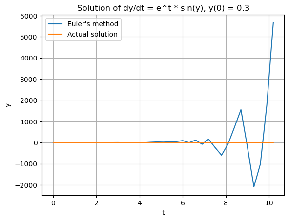
If we change our initial value only slightly from 0.3 to 0.302 then we get a completely different, yet distinctively turbulent chart:

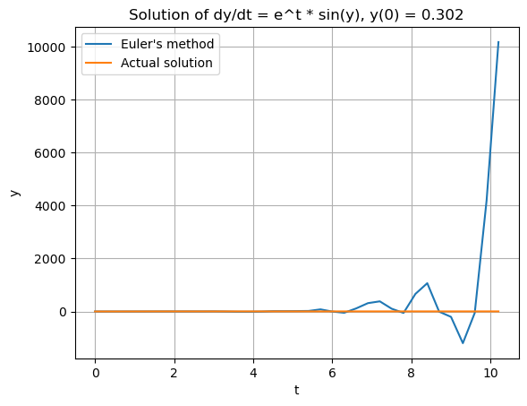
This perfectly demonstrates the sensitivity to initial conditions we talked about earlier. We see this divergence for a few key reasons:

• Non-linearity: Our differential equation is non-linear. The rate of change of y depends not only on y itself but also on its product with \(e^t\). This mathematical relationship introduces an exponential amplification of small variations.
• Discretization: Euler's method approximates a continuous derivative using discrete steps over a finite time interval (dt). This introduces an inherent truncation error at every single step, even with perfect initial conditions.
• The Chaotic Nature: The combination of non-linearity and error amplification makes the system highly sensitive to where it starts. Tiny errors grow exponentially, leading to drastically different trajectories for nearly identical starting points.

The Real "Butterfly Effect" and the Lorenz Attractor

With all of this in mind, we can finally return to the butterfly effect not as it is misunderstood, but as it actually is.

The term "butterfly effect" was coined to describe how minor updates to a state in a deterministic, non-linear system can result in massive differences down the line. Dr. Edward Lorenz discovered this entirely by accident while running a simplified computer model of the weather. He wanted to re-examine a specific sequence, so he restarted the simulation mid-run, typing in the initial conditions from a printout. To save space, the printout rounded the numbers to three decimal places (0.506) instead of the full six digits (0.506127) the computer used internally. That tiny, seemingly inconsequential difference of less than 0.03% completely decoupled the second run from the first, generating a totally different weather forecast. Lorenz famously noted that this meant the exact path and timing of a tornado could be influenced by minor perturbations, like a distant butterfly flapping its wings weeks prior.

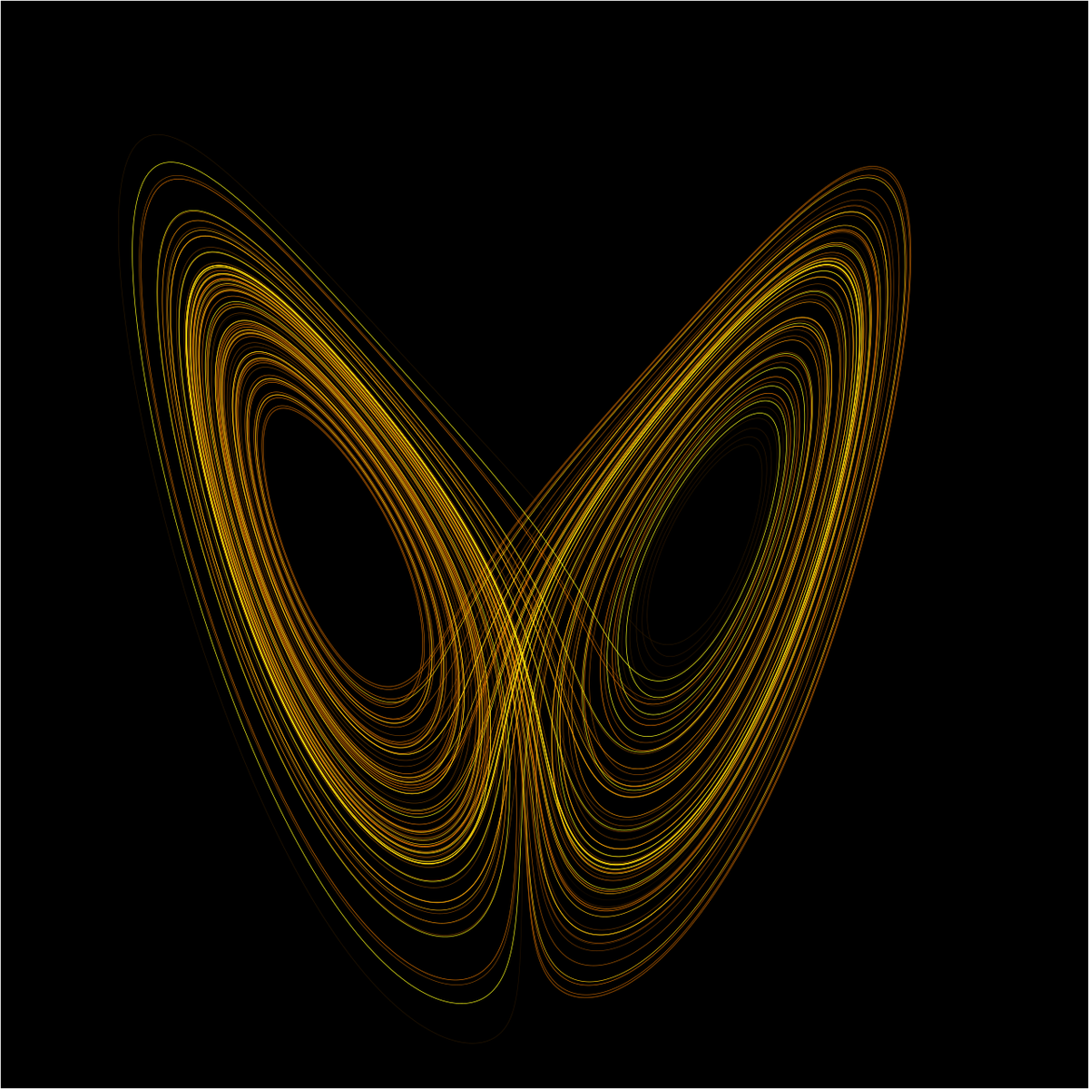
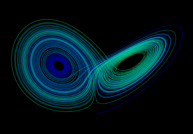
To visualize this deterministic chaos, Lorenz plotted the variables of his simplified weather model in 3D space. The resulting shape created what is now known as a Lorenz attractor. which according to mathematician E.W. Weisstein, arises in a "simplified system of equations describing the two-dimensional flow of fluid of uniform depth." An attractor is simply a set of states toward which a system tends to evolve over time. When you map Lorenz's equations, the coordinates trace out an infinite, non-repeating loop that looks like the wings of a butterfly.

To see this in Python, we can define the Lorenz system a set of three coupled, first-order ordinary differential equations:
$$ du/dt = \sigma (v-u) $$

$$dv/dt = \rho u - v - uw$$

$$dw/dt = uv - \beta w$$

(Note: You will need matplotlib, numpy, and scipy installed to run this code.)

import numpy as np
from scipy.integrate import solve_ivp
import matplotlib.pyplot as plt
from mpl_toolkits.mplot3d import Axes3

WIDTH = 1000
HEIGHT = 750
DPI = 100

# Lorenz paramters and initial conditions.
sigma = 10 
beta = 2.667
rho = 28
u0 = 0 
v0 = 1
w0 = 1.05

# Maximum time point and total number of time points.
tmax = 100
n = 10000

def lorenz(t, X, sigma, beta, rho):
    """The Lorenz equations."""
    u, v, w = X
    up = -sigma*(u - v)
    vp = rho*u - v - u*w
    wp = -beta*w + u*v
    return up, vp, wp

# Integrate the Lorenz equations.
soln = solve_ivp(lorenz, (0, tmax), (u0, v0, w0), args=(sigma, beta, rho),
                 dense_output=True)

# Interpolate solution onto the time grid, t.
t = np.linspace(0, tmax, n)
x, y, z = soln.sol(t)

# Plot the Lorenz attractor using a Matplotlib 3D projection.
fig = plt.figure(facecolor='k', figsize=(WIDTH/DPI, HEIGHT/DPI))
ax = fig.gca(projection='3d')
ax.set_facecolor('k')
fig.subplots_adjust(left=0, right=1, bottom=0, top=1)

# Make the line multi-coloured by plotting it in segments of length s which
# change in colour across the whole time series.
s = 10
cmap = plt.cm.winter
for i in range(0,n-s,s):
    ax.plot(x[i:i+s+1], y[i:i+s+1], z[i:i+s+1], color=cmap(i/n), alpha=0.4)

# Remove all the axis clutter, leaving just the curve.
ax.set_axis_off()

plt.savefig('lorenz.png', dpi=DPI)
plt.show()

Special shout out to Christian Hill over at SciPython for the original script rendering this attractor.

When you run this application, it generates the beautiful, infinite "Butterfly Chart" that visually defines modern Chaos Theory:

What is Chaos Theory Good For?

At this point, you might be saying, "This all sounds very interesting, but what is it actually good for?" Beyond proving that weather forecasting is fundamentally difficult, chaos math plays a massive role in modern science and technology:

• Meteorology: It forms the backbone of probabilistic ensemble forecasting. Because tiny variations drastically alter long-term outcomes, meteorologists run dozens of simultaneous models with slight adjustments to chart the most likely paths of major storms.
• Aerodynamics & Engineering: Chaos theory helps model turbulent airflow over aircraft wings and fluid dynamics inside burning turbofan engines. Conversely, engineers deliberately use chaos equations to design micro-mixers that rapidly blend fluids at microscopic scales.
• Medicine & Biology: It is used to model complex biological rhythms, such as irregular heartbeats (arrhythmias) or erratic epileptic brain activity, enabling better diagnostic tools and medical treatments.
• Cybersecurity: Chaotic mathematical models are frequently applied to cryptography to generate highly unpredictable, secure sequences for data encryption and random number generation.

Any one of these topics could be a deep-dive post in itself. But for now, you are officially acquainted with the basics of Chaos Theory as it really is. Stay tuned to see what else we’re cooking up here at The Puttering Dev!